Learn Analog Circuits with Zundamon

Episode 3

Transconductance and the Common-Source Amplifier

The key to amplifying a signal with a MOSFET is transconductance gm and the small-signal model.

Watch on YouTube (11:44)
  • Shikoku Metan (explains)
  • Zundamon (asks)

1Intro: a larger input distorts the waveform

Zundamon

My amplifier homework needs resubmitting! A bigger input distorted the output!
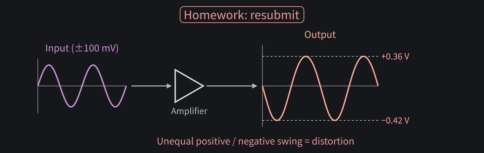
Illustration: My amplifier homework needs resubmitting! A bigger input distorted the output!

Figure 1

Shikoku Metan

Separate the DC operating point from the small signal around it.

Shikoku Metan: The keys are gm and the small-signal model. Then we'll build a common-source stage.

Illustration: The keys are gm and the small-signal model. Then we'll build a common-source stage.
Figure 2

Zundamon

Please! This time I want to explain it properly, nanoda!

Illustration: Please! This time I want to explain it properly, nanoda!
Figure 3

2Bias point and small signals (uppercase and lowercase notation)
Shikoku Metan

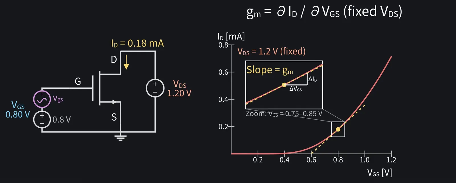
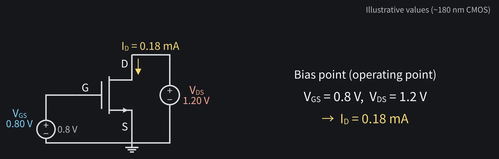
Back to episode one's test circuit. Keep VDS fixed at 1.2 V.

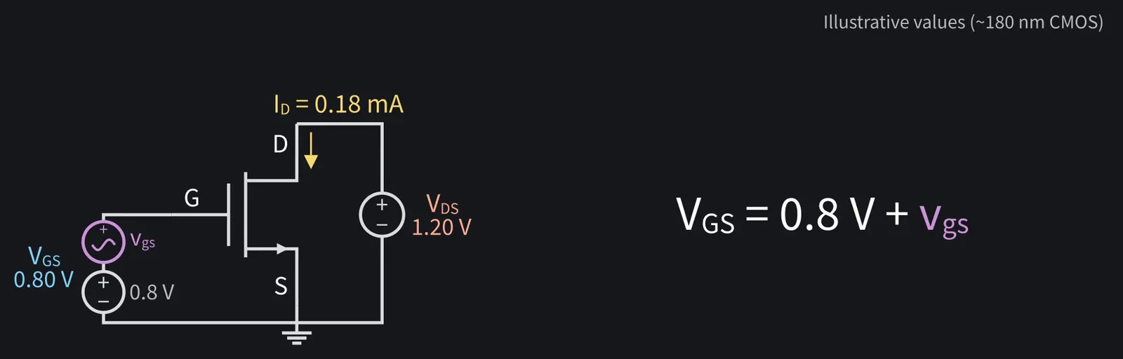
Shikoku Metan: The DC gate-source voltage is 0.8 V. This operating point is the bias point.

Illustration: The DC gate-source voltage is 0.8 V. This operating point is the bias point.
Figure 4

Shikoku Metan

Add a small signal vgs: the total VGS is 0.8 V plus vgs.

Illustration: Add a small signal vgs: the total VGS is 0.8 V plus vgs.
Figure 5

ZundamonQuestion

What's the difference between uppercase and lowercase?
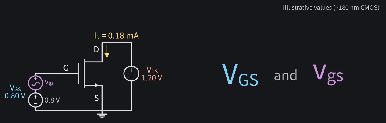
Illustration: What's the difference between uppercase and lowercase?
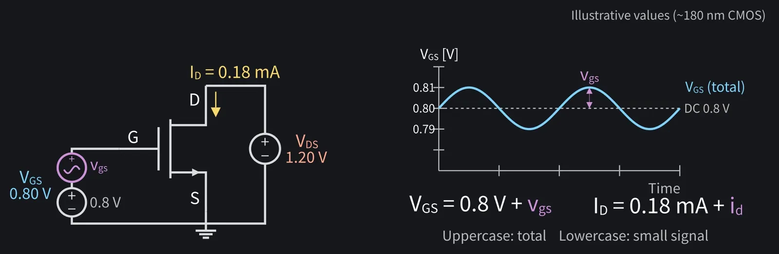
Figure 6

Shikoku Metan

Uppercase is the total; lowercase is the small signal. Likewise, ID and id.

Illustration: Uppercase is the total; lowercase is the small signal. Likewise, ID and id.
Figure 7

Shikoku Metan

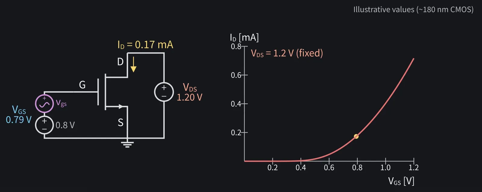
On the ID–VGS curve, the point moves just a little around the bias point.

Illustration: On the ID–VGS curve, the point moves just a little around the bias point.
Figure 8

Shikoku Metan

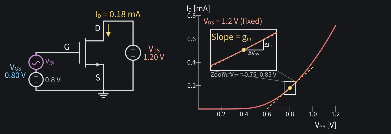
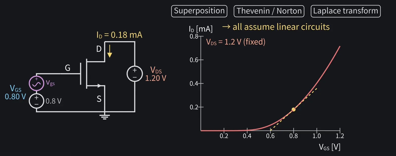
Zoom in around the bias point, and the curve looks almost straight.

Zundamon

Even a curve looks straight over a narrow range!

Shikoku Metan

Approximate it with this tangent, and ordinary linear circuit theory applies.

3Why use both large-signal and small-signal analysis?

ZundamonQuestion

Can't circuit theory solve the original curve?
Shikoku Metan

Superposition, Thévenin's theorem, Laplace transforms: they all assume a linear circuit.

Illustration: Superposition, Thévenin's theorem, Laplace transforms: they all assume a linear circuit.
Figure 9

Shikoku Metan

A MOSFET is nonlinear: doubling VGS doesn't simply double ID.

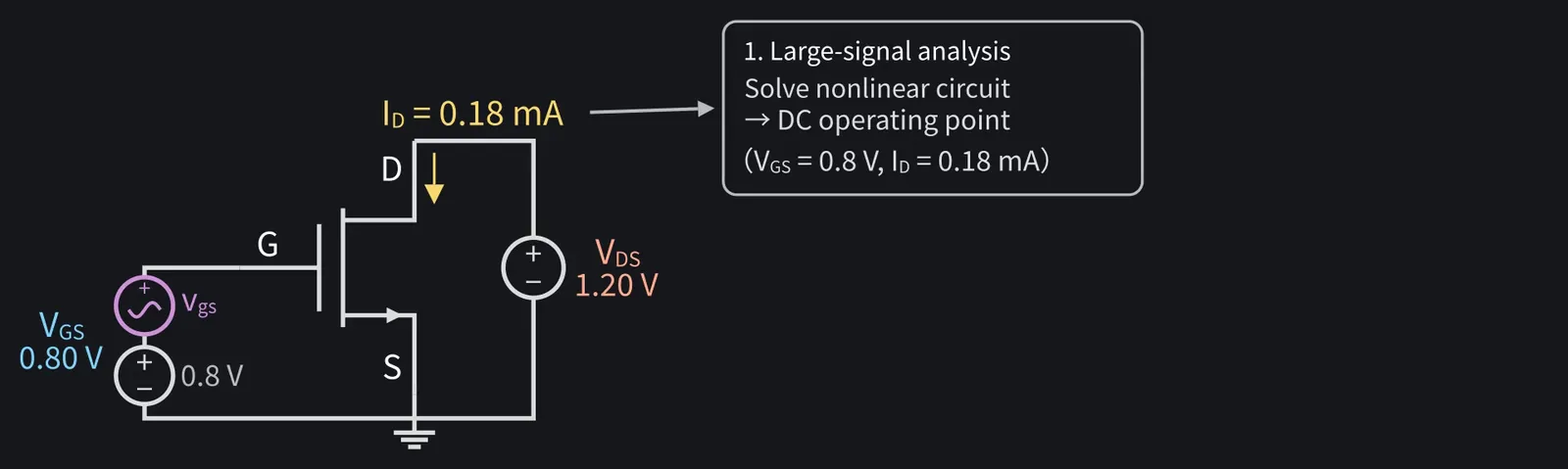
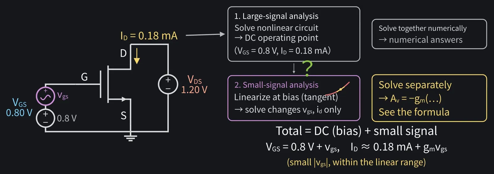
Shikoku Metan: So use two steps. Large-signal analysis first finds the nonlinear DC bias point.

Illustration: So use two steps. Large-signal analysis first finds the nonlinear DC bias point.
Figure 10

Shikoku Metan

Then small-signal analysis: linearize the circuit at that point and solve only for the changes.

ZundamonQuestion

I don't get it. Why solve the same circuit twice?
Shikoku Metan

Numerically, you can solve it all at once. Splitting it reveals gain formulas.

Shikoku Metan: The total is DC plus the small signal, within the range where linearization works.

Illustration: The total is DC plus the small signal, within the range where linearization works.
Figure 11

4Defining gm: the tangent slope

Shikoku Metan

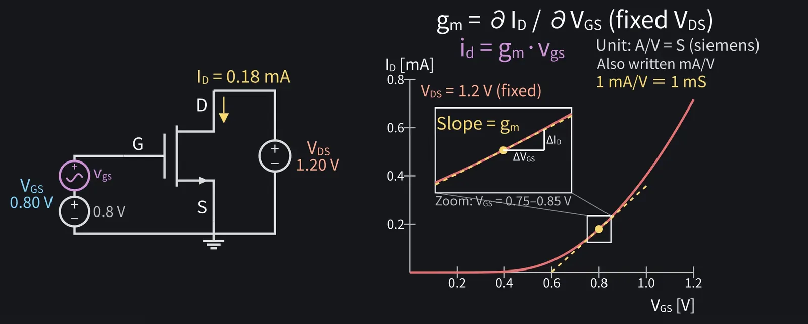
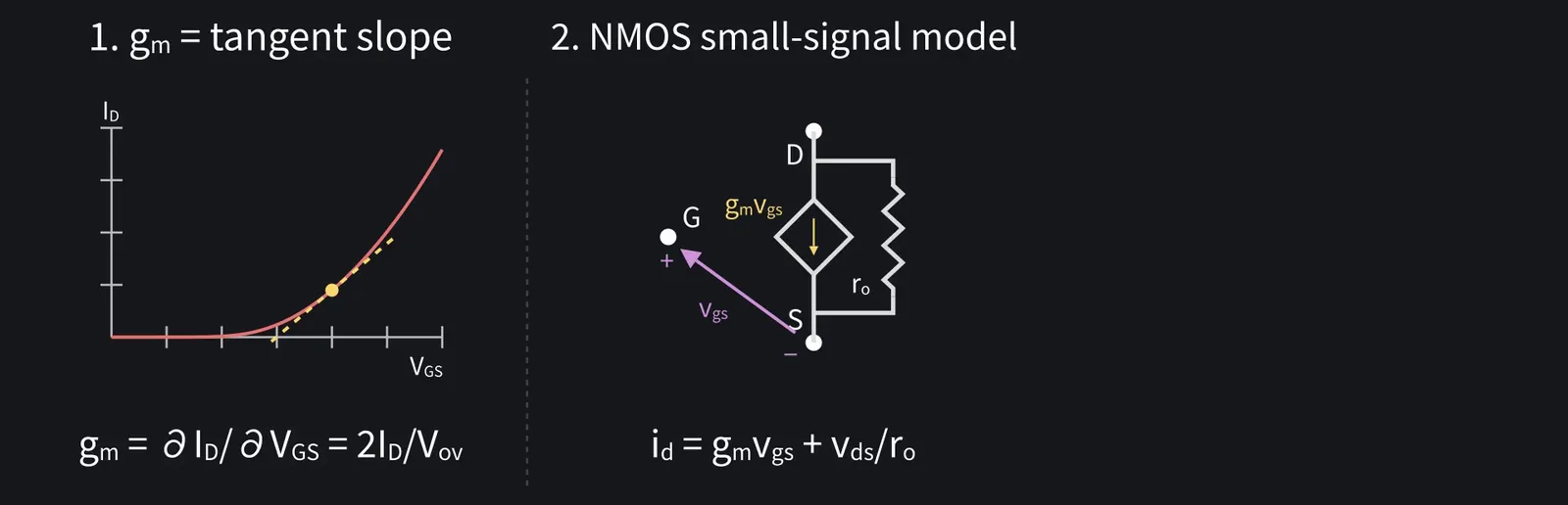
Back to the tangent. Its slope is called transconductance, gm.

Illustration: Back to the tangent. Its slope is called transconductance, gm.
Figure 12

Shikoku Metan

gm = ∂ID/∂VGS, differentiating while VDS stays fixed.

Illustration: gm = ∂ID/∂VGS, differentiating while VDS stays fixed.
Figure 13

Shikoku Metan

So id=gm·vgs: a voltage change produces a current change.

Shikoku Metan: The unit is siemens, S. One mA/V equals one mS.

Illustration: The unit is siemens, S. One mA/V equals one mS.
Figure 14

5gm = K·Vov=2·ID/Vov in saturation
Shikoku Metan

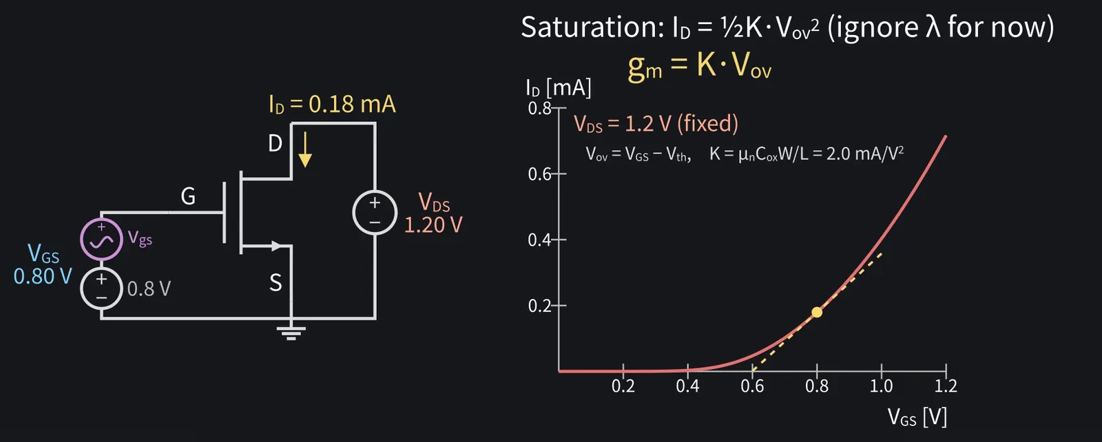
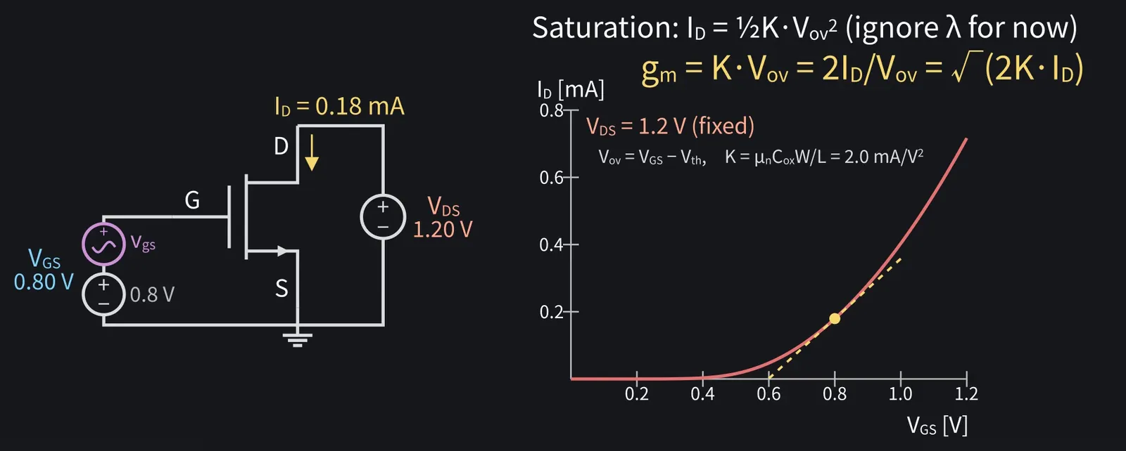
In saturation, ID = ½K·Vov², where Vov=VGS−Vth. Ignore channel-length modulation for now.

Shikoku Metan: Differentiate with respect to VGS: gm = K·Vov, proportional to overdrive.

Illustration: Differentiate with respect to VGS: gm = K·Vov, proportional to overdrive.
Figure 15

Shikoku Metan

Using ID instead, gm=2·ID/Vov, or equivalently √(2K·ID).

Illustration: Using ID instead, gm = 2·ID/Vov, or equivalently √(2K·ID).
Figure 16

Shikoku Metan

Use the bias-point values of ID and Vov in these formulas.

6Numerical example and the small-signal condition

Shikoku Metan

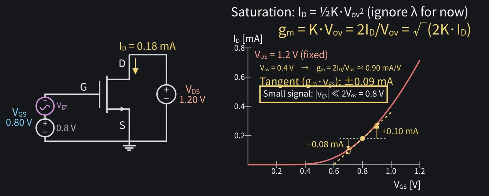
Let's calculate with episode one's model: K = 2 mA/V², Vth=0.4 V, λ = 0.1 V⁻¹. At the bias point, ID is about 0.18 mA.

Shikoku Metan: Vov is 0.4 V, so gm=2·ID/Vov gives about 0.9 mA/V.

ZundamonQuestion

But K·Vov gives 0.8 mA/V. Why don't they match?

Shikoku Metan

Sharp eye. The difference is the factor (1 + λVDS) = 1.12; the 2·ID/Vov form includes it, K·Vov doesn't.

ZundamonQuestion

How small does a small signal need to be?

Shikoku Metan

A 10 mV input change gives about 9 µA, almost exactly gm·vgs.

ZundamonQuestion

What about a 100 mV change?
Shikoku Metan

Upward gives about +0.10 mA; downward about −0.08 mA. They're unequal.

Shikoku Metan: vgs must be much smaller than twice Vov, which is 0.8 V here. That's the small-signal condition.

Illustration: vgs must be much smaller than twice Vov, which is 0.8 V here. That's the small-signal condition.
Figure 17

7The NMOS small-signal equivalent circuit: four steps
Shikoku Metan

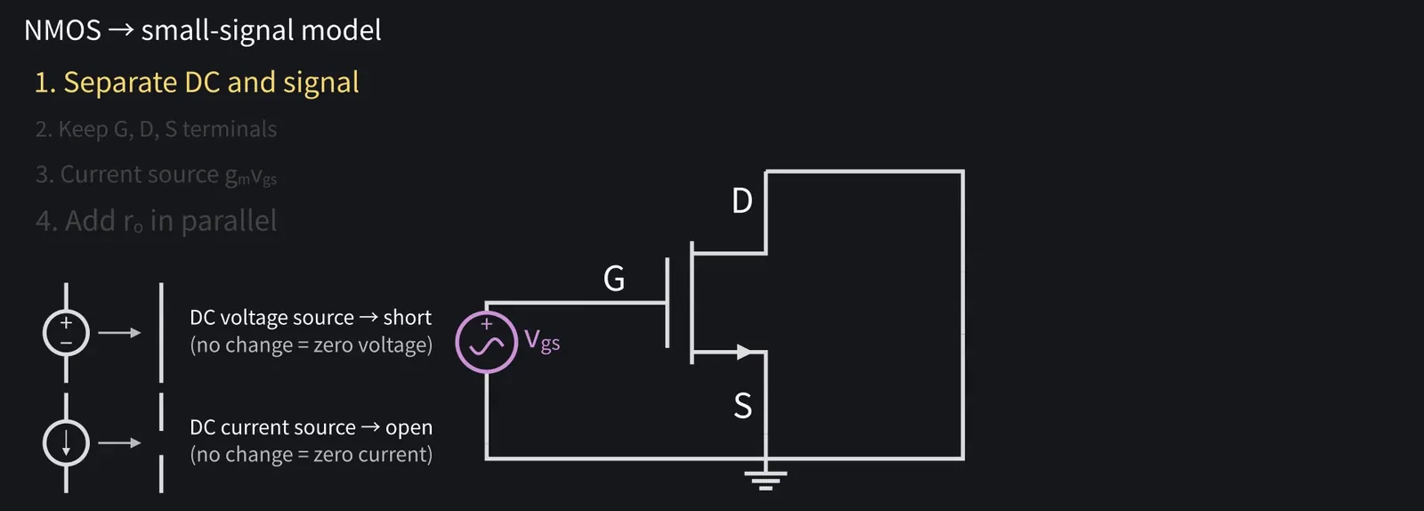
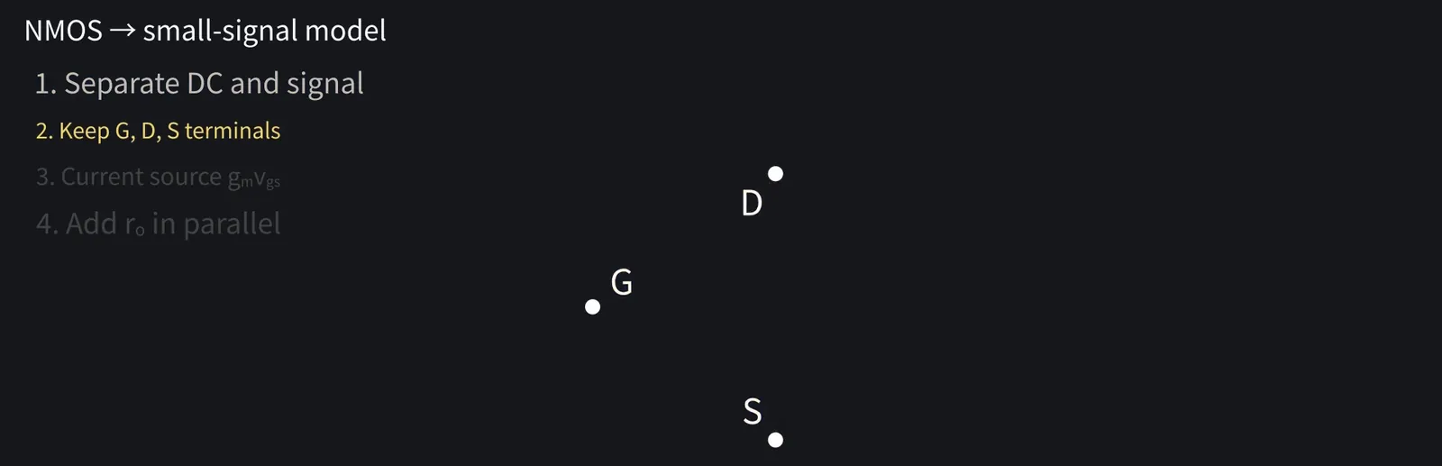
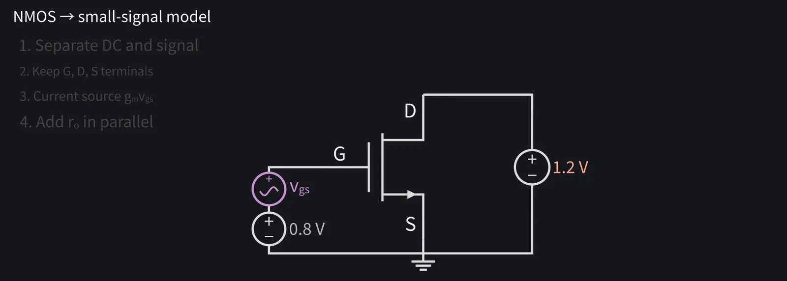
Let's build the NMOS small-signal equivalent, one step at a time.

Illustration: Let's build the NMOS small-signal equivalent, one step at a time.
Figure 18

Shikoku Metan

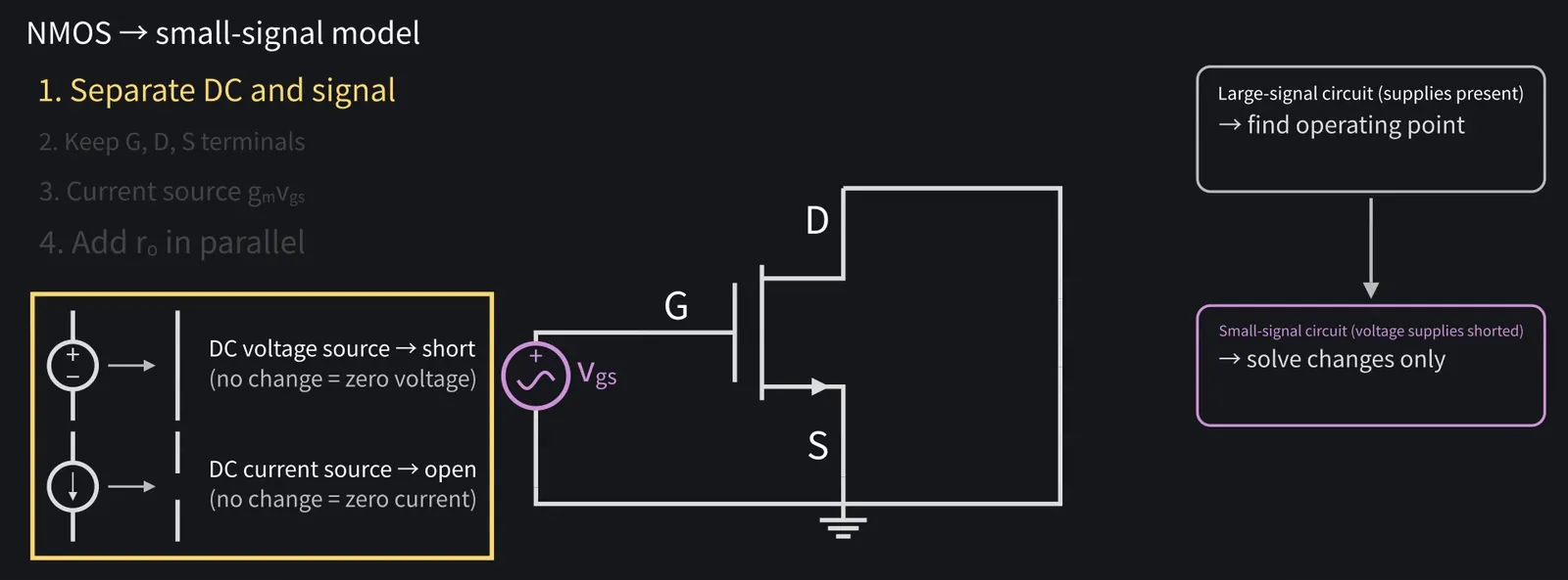
Step one: separate the DC bias from the small signal.

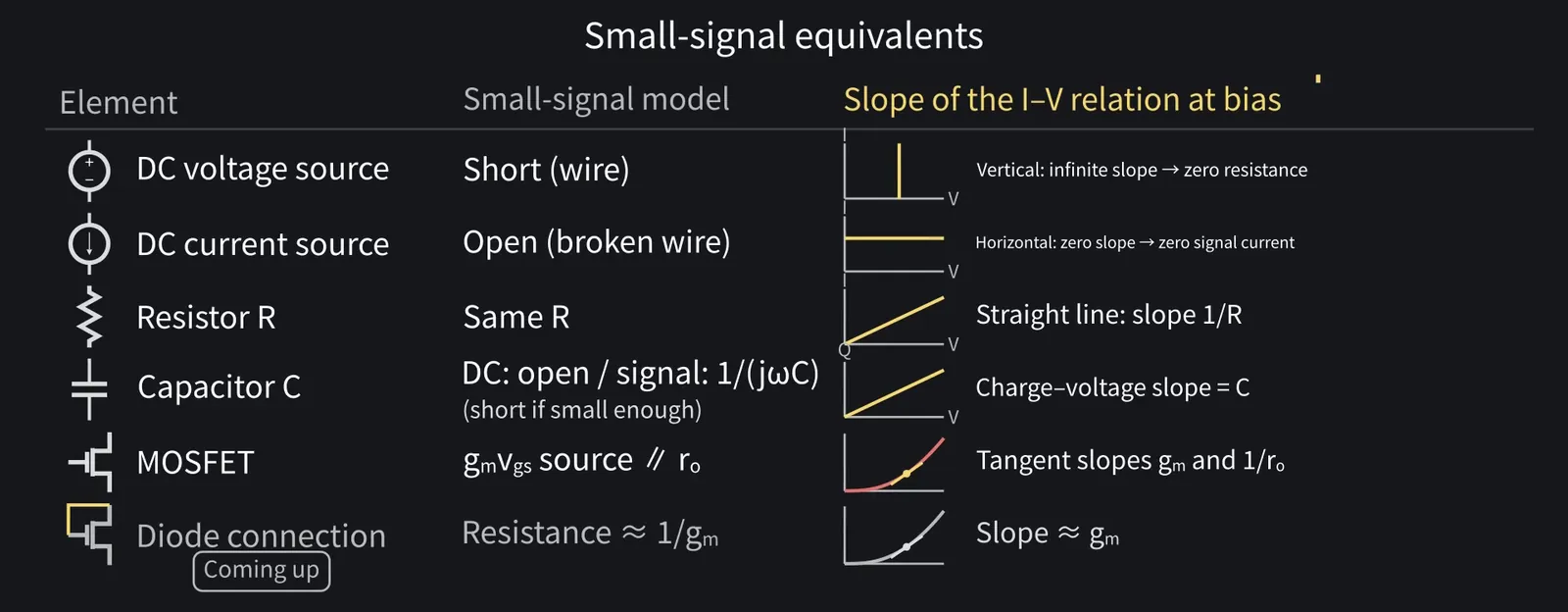
Shikoku Metan: A DC voltage source has no signal voltage, so replace it with a short to ground.

Shikoku Metan: A DC current source has no signal current, so replace it with an open circuit.

Illustration: A DC current source has no signal current, so replace it with an open circuit.
Figure 19

Zundamon

Zero change! Zero voltage is a short, zero current is an open!

Zundamon: Wait! Won't removing the supply turn the transistor off?
Shikoku Metan

Only in the small-signal circuit. Large-signal analysis already found the bias.

Illustration: Only in the small-signal circuit. Large-signal analysis already found the bias.
Figure 20

Shikoku Metan

Its effects remain in gm and ro. The supply's role hasn't disappeared.

Shikoku Metan: A resistor has the same R for changes in voltage and current, so keep it.

ZundamonQuestion

What about a capacitor?
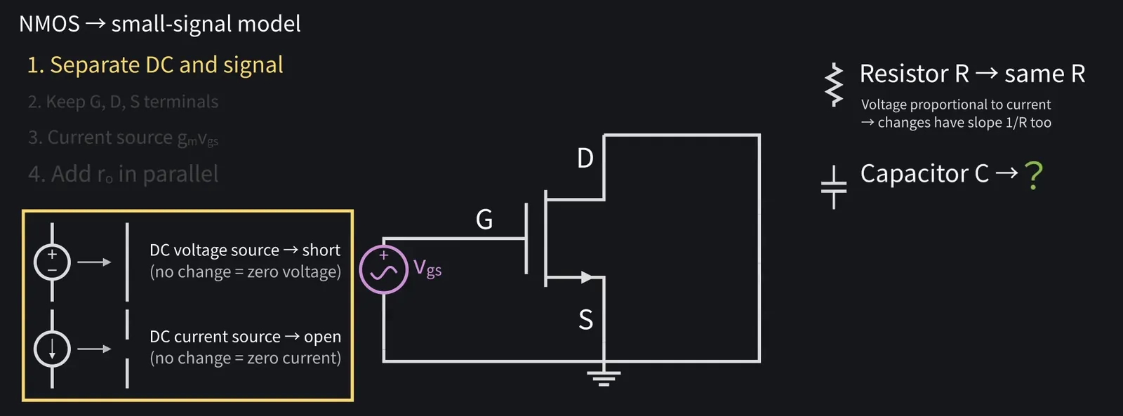
Illustration: What about a capacitor?
Figure 21

Shikoku Metan

Open for DC. For a small signal, its impedance is 1/(jωC).

Shikoku Metan: The larger the capacitance and the higher the frequency, the smaller it gets. If it's much smaller than the surrounding resistances, treat it as a short.

Shikoku Metan: Step two: keep the same three terminals, gate, drain, and source.

Illustration: Step two: keep the same three terminals, gate, drain, and source.
Figure 22

Shikoku Metan

No current flows into the gate, so gate to source is open.

Shikoku Metan: vgs is the gate-source signal voltage, positive at the gate.

Shikoku Metan: Step three: add a current source gm·vgs directed from drain to source.

Zundamon

That's the dependent source from episode one!
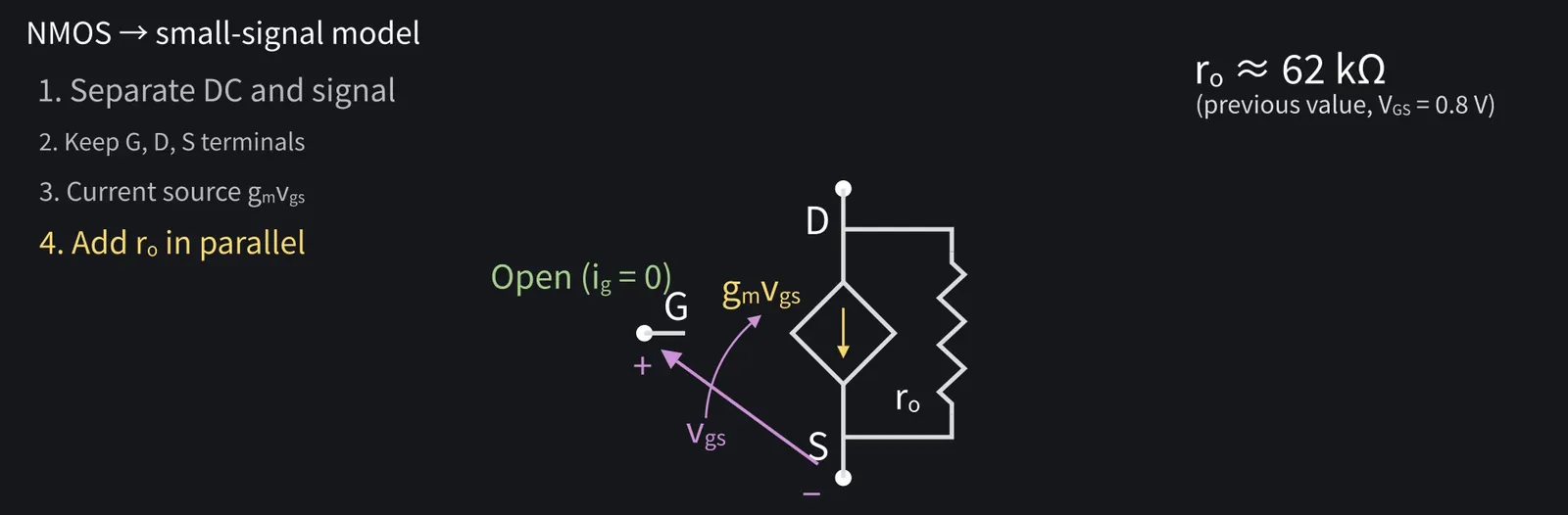
Shikoku Metan

Step four: add ro in parallel to represent channel-length modulation.

Shikoku Metan: As last time, at VGS=0.8 V, ro is about 62 kΩ.

Illustration: As last time, at VGS = 0.8 V, ro is about 62 kΩ.
Figure 23

Shikoku Metan

Together, id=gm·vgs+vds/ro, where vds is the drain-source signal voltage.

Shikoku Metan: The body is tied to the source, so the body-effect contribution is zero.

Shikoku Metan: We're also omitting MOSFET capacitances for this low-frequency model.

Shikoku Metan: In the test circuit, short the VDS supply. Then vds=0 and id=gm·vgs.

Shikoku Metan: Here's the replacement table. Each model uses the slope at the bias point.

Illustration: Here's the replacement table. Each model uses the slope at the bias point.
Figure 24

8Intrinsic gain gm·ro

Shikoku Metan

gm·ro is intrinsic gain: a guide to the gain available from one transistor.

Illustration: gm·ro is intrinsic gain: a guide to the gain available from one transistor.
Figure 25

Shikoku Metan

Here it's about 56. Using ro≈1/(λID), you get the estimate 2/(λVov), about 50.

9Common-source amplifier: load line and transfer curve
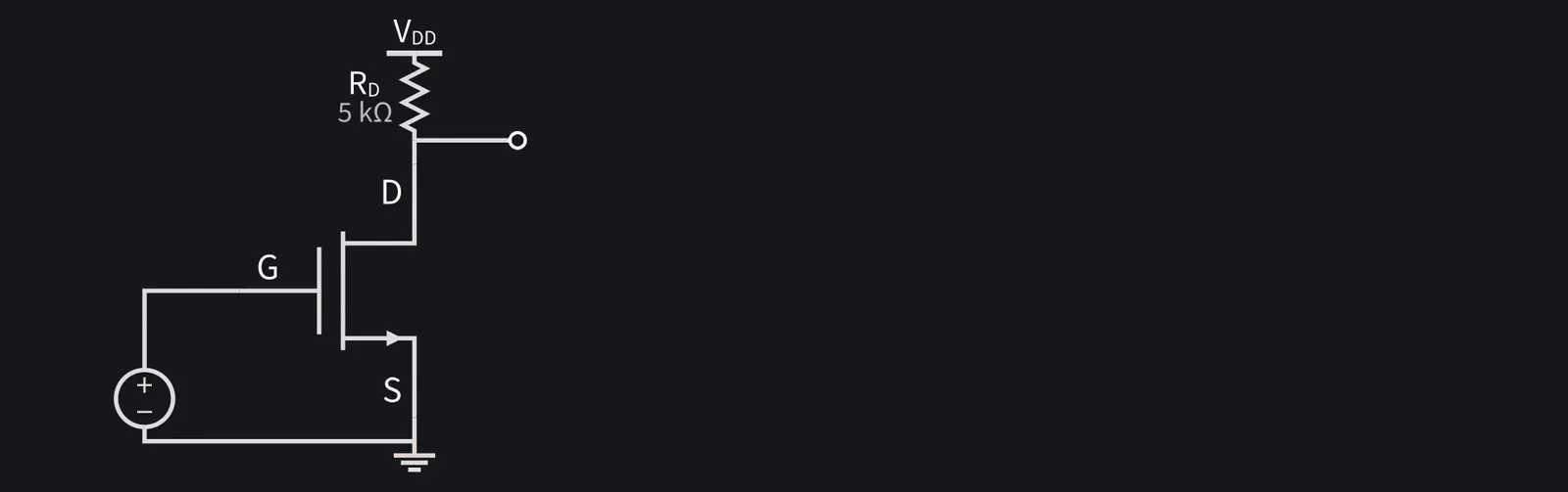
Shikoku Metan

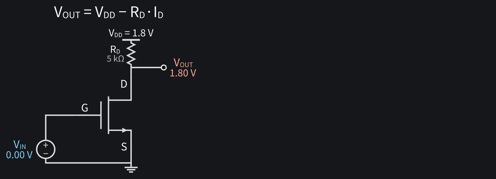
Now the common-source amplifier: RD and VDD at the drain, source grounded.

Illustration: Now the common-source amplifier: RD and VDD at the drain, source grounded.
Figure 26

Shikoku Metan

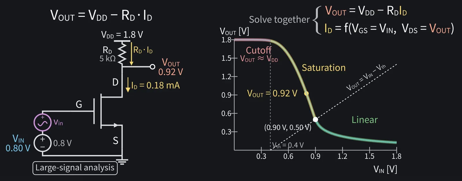
Use VDD=1.8 V and RD=5 kΩ, with VIN at the gate.

Shikoku Metan: The drain voltage is the output: VOUT=VDD−RD·ID.

Illustration: The drain voltage is the output: VOUT = VDD − RD·ID.
Figure 27

ZundamonQuestion

More ID means a bigger drop across RD and a lower output?
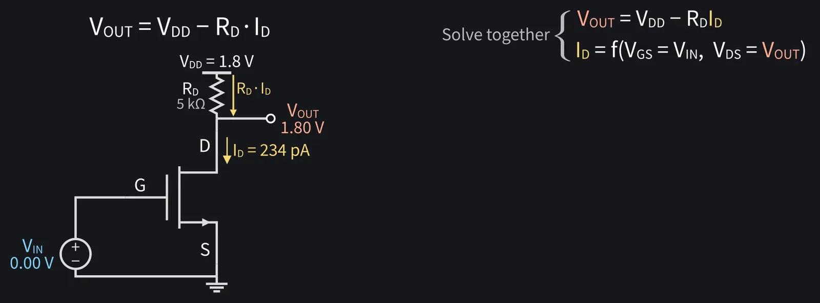
Shikoku Metan

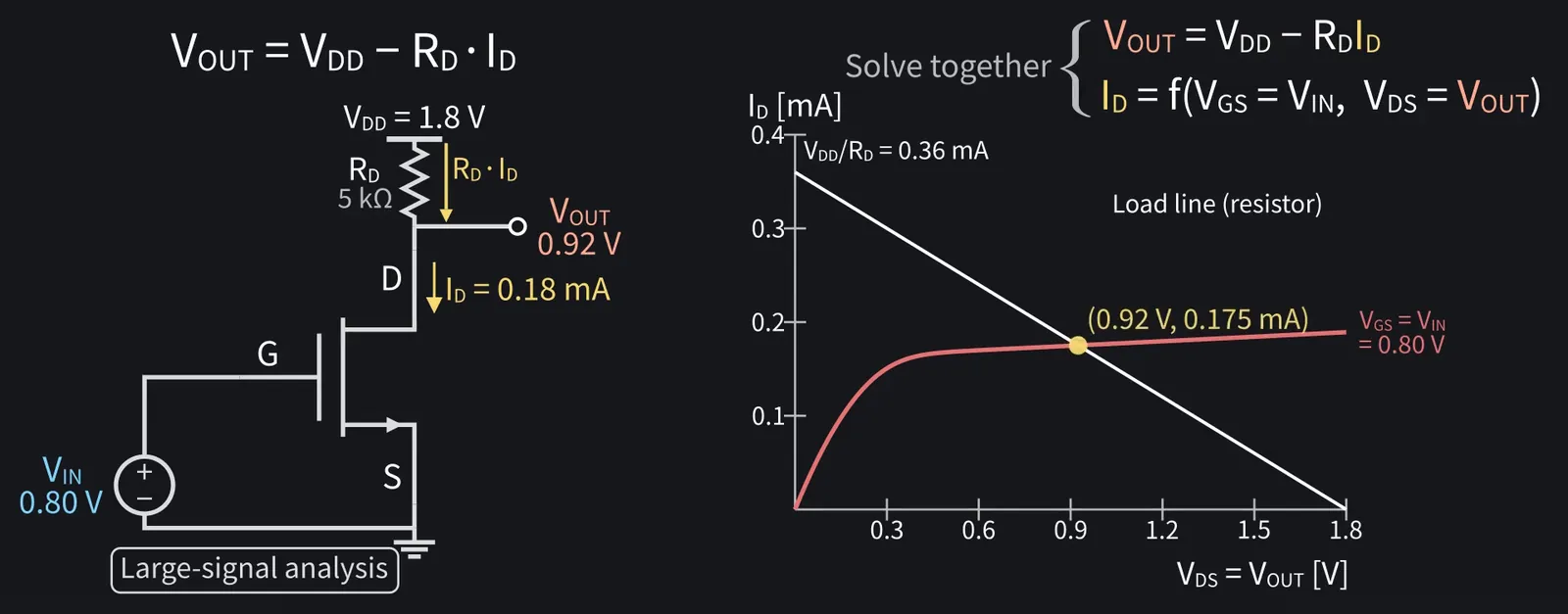
Right. But ID also depends on VDS, which is VOUT, so solve the two equations together.

Illustration: Right. But ID also depends on VDS, which is VOUT, so solve the two equations together.
Figure 28

Shikoku Metan

The current equation is nonlinear. Solving it numerically is large-signal analysis.

Shikoku Metan: On this graph, find the intersection with RD's straight line, the load line.

Illustration: On this graph, find the intersection with RD's straight line, the load line.
Figure 29

Zundamon

Raise VIN and the MOSFET's curve moves up, so the intersection with the load line moves left!
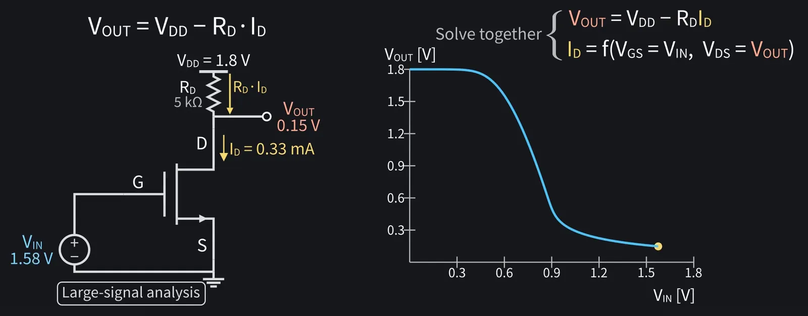
Shikoku Metan

Find VOUT for each VIN and join the points to get this transfer curve.

Illustration: Find VOUT for each VIN and join the points to get this transfer curve.
Figure 30

Shikoku Metan

Below Vth, current is tiny, so VOUT stays close to VDD.

Shikoku Metan: Above Vth, the device enters saturation and VOUT drops sharply.

Shikoku Metan: The boundary is the line VOUT=VIN−Vth. Near VIN=0.9 V and VOUT=0.5 V, the curve crosses it into the linear region.

Shikoku Metan: Bias at VIN=0.8 V along that steep part: VOUT is about 0.92 V.

Illustration: Bias at VIN = 0.8 V along that steep part: VOUT is about 0.92 V.
Figure 31

Shikoku Metan

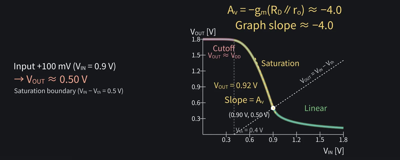
The slope here is the small-signal voltage gain, Av.

10Small-signal circuit and Av = −gm(RD∥ro)
Shikoku Metan

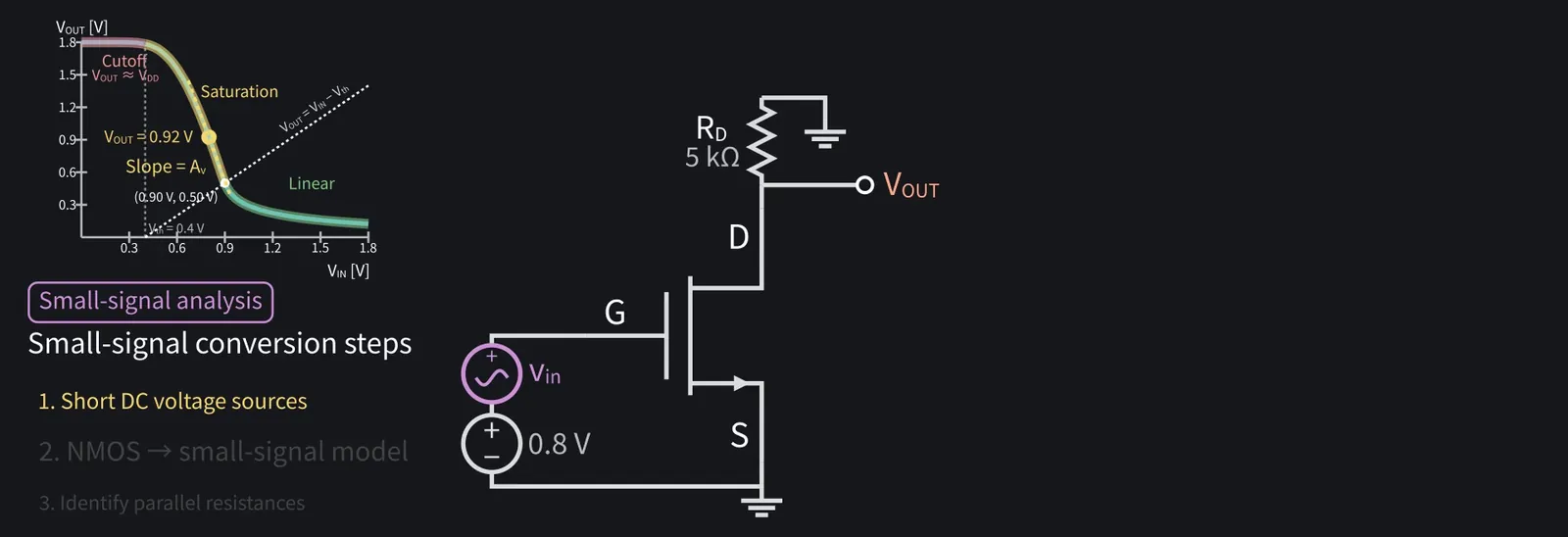
Now small-signal analysis. Transform the circuit to derive that gain.

Shikoku Metan: Step one: VDD is a DC voltage source, so short it to signal ground.

Illustration: Step one: VDD is a DC voltage source, so short it to signal ground.
Figure 32

Shikoku Metan

Short the input's 0.8 V DC component too. Only vin remains.

Zundamon

So the top of RD connects to ground!
Shikoku Metan

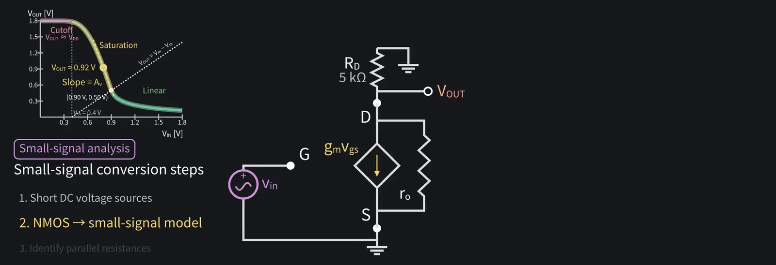
Step two: replace the NMOS with its small-signal model.

Illustration: Step two: replace the NMOS with its small-signal model.
Figure 33

Shikoku Metan

The gate has vin and the source is grounded, so vgs=vin.

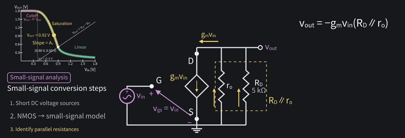
Shikoku Metan: Step three: both ro and RD connect between output and ground.

Zundamon

The same two nodes! They're in parallel!
Shikoku Metan

Redraw it as a gm·vin current source with RD∥ro.

Shikoku Metan: The source draws current from the output: vout = −gm·vin·(RD∥ro).

Illustration: The source draws current from the output: vout = −gm·vin·(RD∥ro).
Figure 34

Shikoku Metan

So Av = −gm(RD∥ro). The minus sign means the output moves opposite to the input.

Shikoku Metan: gm is slightly lower here, about 0.87 mA/V, because VDS is now 0.92 V instead of 1.2 V. RD∥ro=5 kΩ∥62 kΩ≈4.6 kΩ, so Av ≈ −4.

Zundamon

It matches the graph's slope!
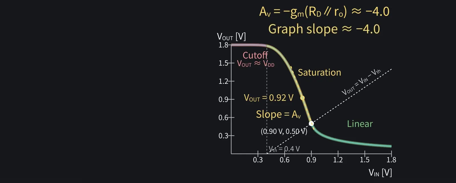
Illustration: It matches the graph's slope!
Figure 35

Shikoku Metan

A 10 mV input gives an inverted output wave of about 40 mV.

11Output swing limits

Shikoku Metan

Output swing is limited, too. A +100 mV input pulls VOUT down to about 0.5 V, right at the edge of saturation.

Illustration: Output swing is limited, too. A +100 mV input pulls VOUT down to about 0.5 V, right at the edge of saturation.
Figure 36

Shikoku Metan

The transistor must remain in saturation throughout the signal swing.

12What each analysis reveals

ZundamonQuestion

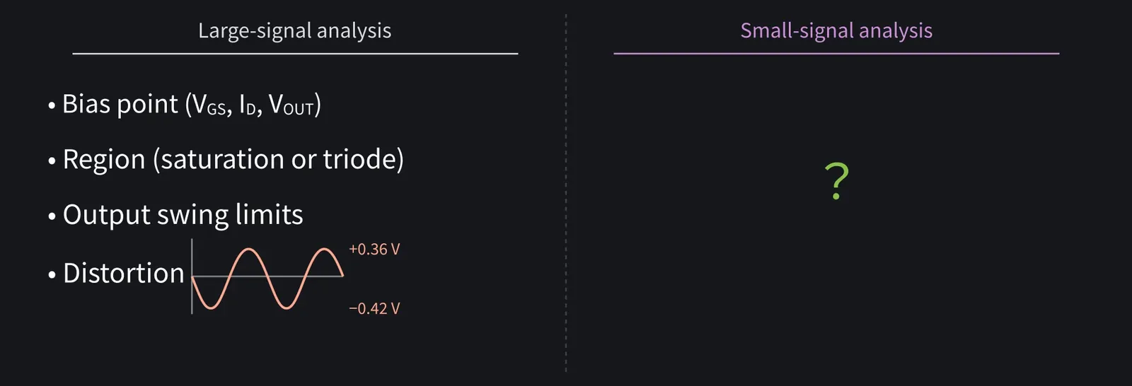
What does each analysis tell us in the end?
Shikoku Metan

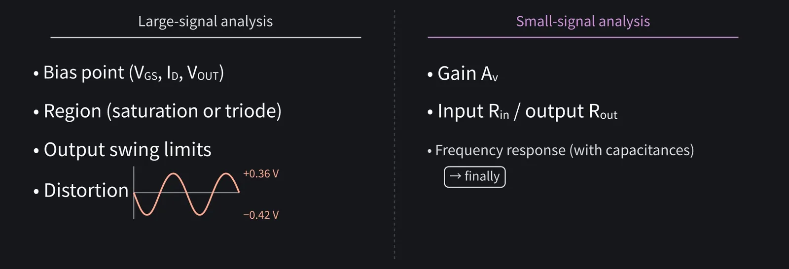
Large-signal analysis gives bias, operating region, swing limits, and distortion.

Illustration: Large-signal analysis gives bias, operating region, swing limits, and distortion.
Figure 37

Shikoku Metan

Small-signal analysis gives gain and resistances, and frequency response with caps.

Illustration: Small-signal analysis gives gain and resistances, and frequency response with caps.
Figure 38

13Solving small-signal circuits efficiently: Rin, Rout, and Gm
Shikoku Metan

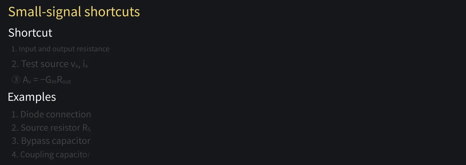
Let's practice some shortcuts for solving small-signal circuits.

Illustration: Let's practice some shortcuts for solving small-signal circuits.
Figure 39

Shikoku Metan

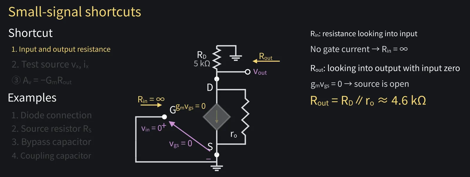
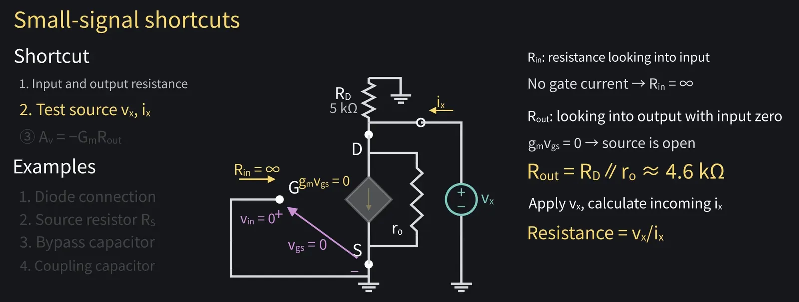
First, the input resistance Rin, seen looking into the input. For common source that's the gate, so it's infinite.

Shikoku Metan: The output resistance Rout is seen looking into the output with the input set to zero: RD∥ro, about 4.6 kΩ.

Illustration: The output resistance Rout is seen looking into the output with the input set to zero: RD∥ro, about 4.6 kΩ.
Figure 40

Shikoku Metan

To find it, connect a test source vx at the output and compute the current ix flowing in. Rout=vx/ix.

Illustration: To find it, connect a test source vx at the output and compute the current ix flowing in. Rout = vx/ix.
Figure 41

Shikoku Metan

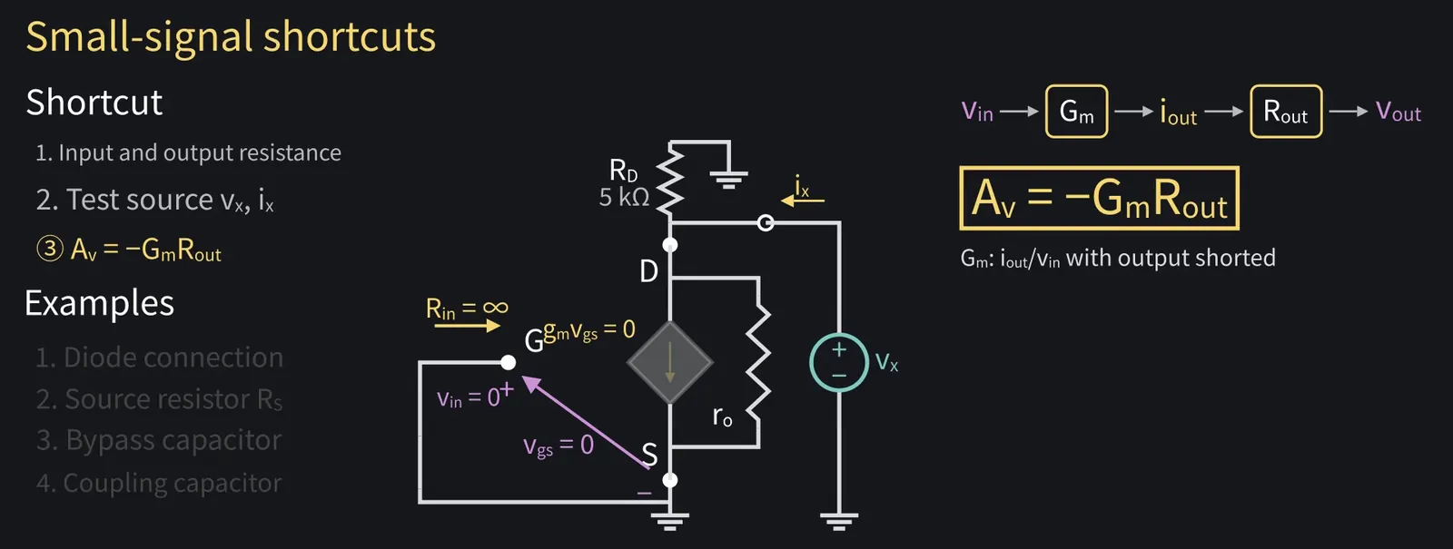
Think of gain as Av = −Gm·Rout: voltage-to-current conversion times resistance.

Illustration: Think of gain as Av = −Gm·Rout: voltage-to-current conversion times resistance.
Figure 42

Zundamon

For common source, Gm=gm, so we immediately get −gm(RD∥ro)!
Shikoku Metan

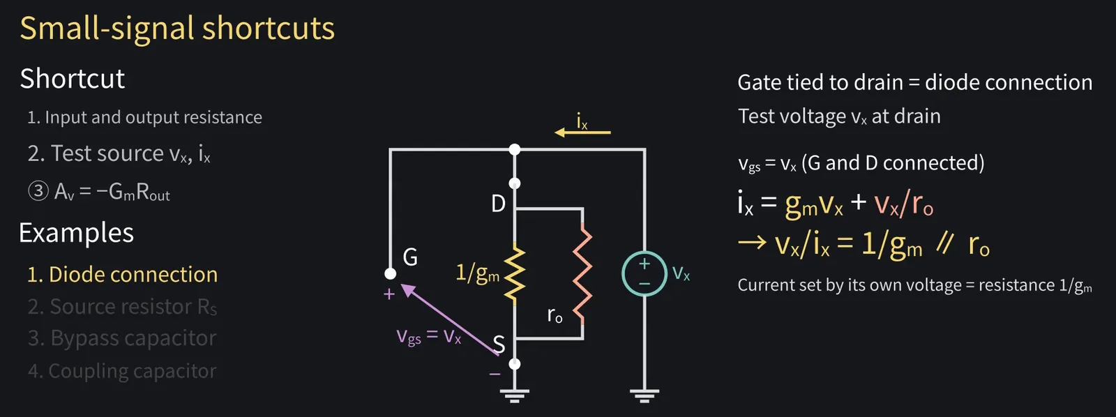
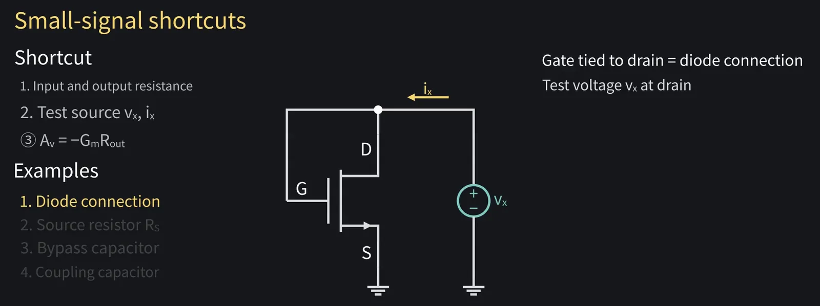
Practice with a MOSFET whose gate and drain are tied: a diode connection.

Illustration: Practice with a MOSFET whose gate and drain are tied: a diode connection.
Figure 43

Shikoku Metan

vgs=vx, so ix=gm·vx+vx/ro. Its resistance is (1/gm)∥ro.

Illustration: vgs = vx, so ix = gm·vx + vx/ro. Its resistance is (1/gm)∥ro.
Figure 44

Shikoku Metan

ro is much larger, so resistance is about 1/gm. We'll use this in episode four.

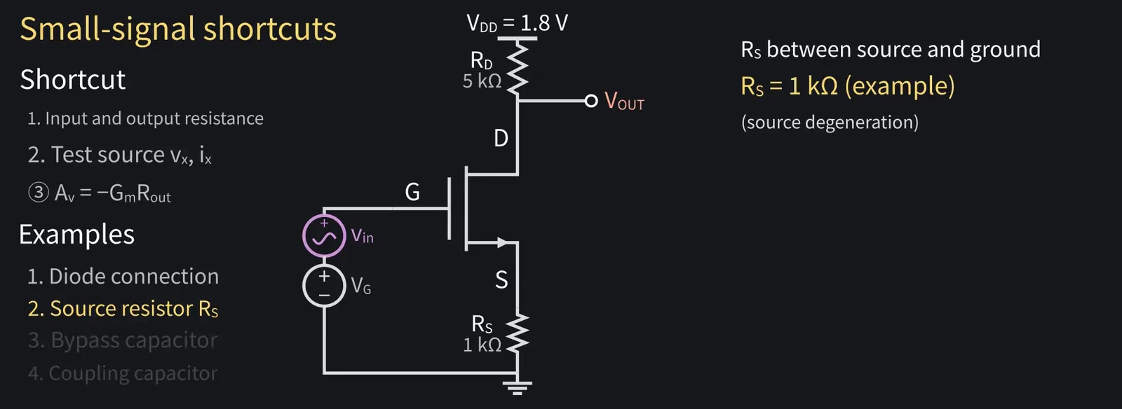
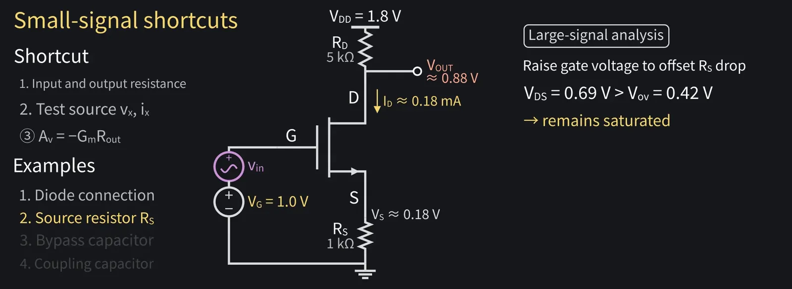
Shikoku Metan: Next, add RS=1 kΩ between the source and ground.

Illustration: Next, add RS = 1 kΩ between the source and ground.
Figure 45

Shikoku Metan

Large signal first. RS drops about 0.18 V, so raise the gate DC to 1.0 V. Then VOUT≈0.88 V, still in saturation.

Illustration: Large signal first. RS drops about 0.18 V, so raise the gate DC to 1.0 V. Then VOUT ≈ 0.88 V, still in saturation.
Figure 46

Shikoku Metan

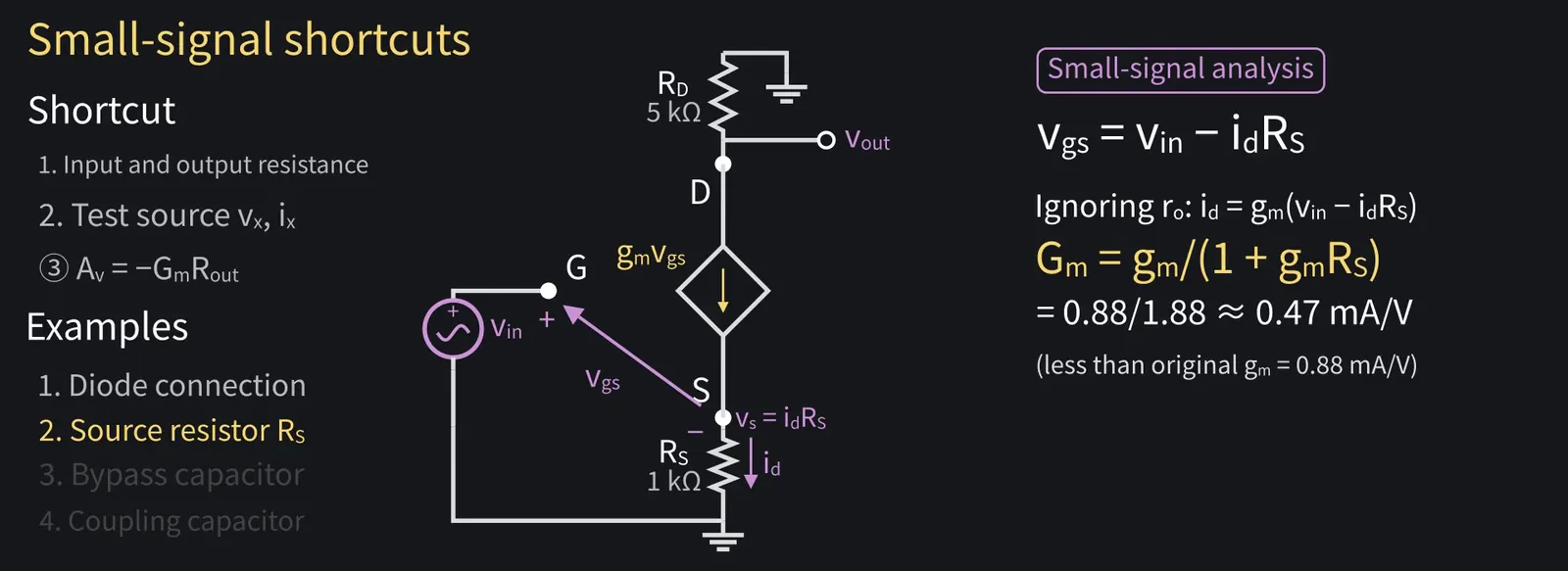
The signal source voltage is id·RS, so vgs=vin−id·RS.

Shikoku Metan: Ignoring ro, Gm=gm/(1+gm·RS), smaller than gm.

Illustration: Ignoring ro, Gm = gm/(1 + gm·RS), smaller than gm.
Figure 47

Shikoku Metan

Av ≈ −RD/(RS+1/gm) ≈ −2.3. The model's slope is about −2.2.

ZundamonQuestion

The gain dropped. What's the advantage?
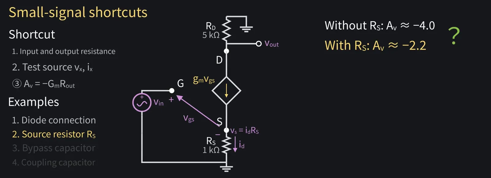
Illustration: The gain dropped. What's the advantage?
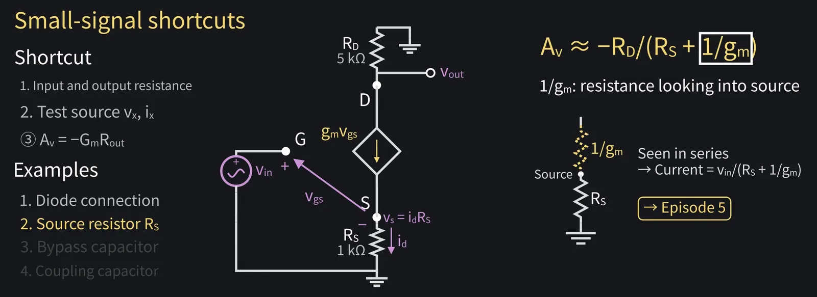
Figure 48

Shikoku Metan

If gm changes by ten percent, the gain changes only about five percent; without RS it would change the full ten. So the output distorts less.

Shikoku Metan: 1/gm is the resistance looking into the source. More in episode five.

Illustration: 1/gm is the resistance looking into the source. More in episode five.
Figure 49

ZundamonQuestion

What if a large capacitor is connected across RS?
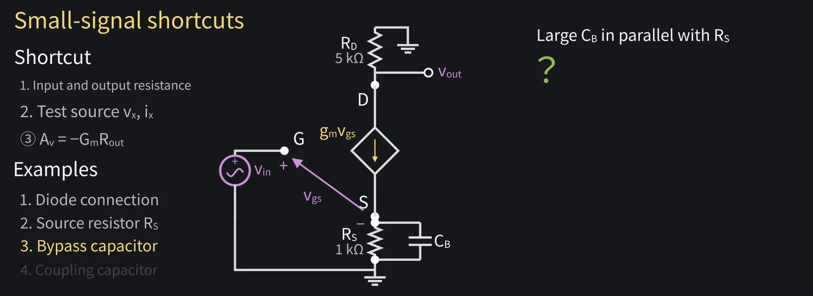
Illustration: What if a large capacitor is connected across RS?
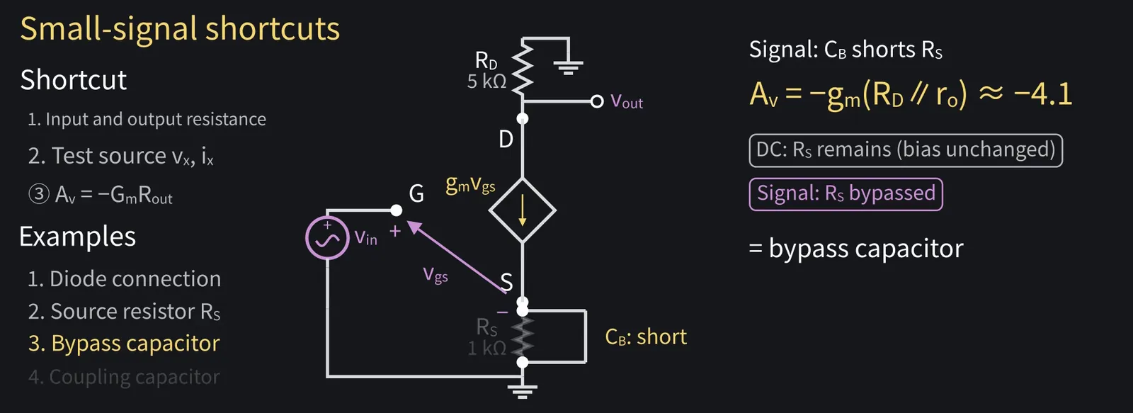
Figure 50

Shikoku Metan

For the signal it shorts RS, restoring gain to about −4. That's a bypass capacitor.

Illustration: For the signal it shorts RS, restoring gain to about −4. That's a bypass capacitor.
Figure 51

ZundamonQuestion

If the signal source has zero DC voltage, how do we keep the gate at 0.8 V?
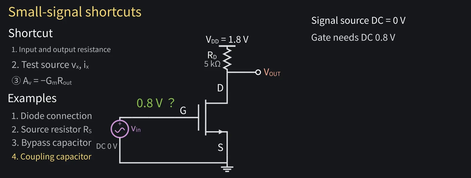
Illustration: If the signal source has zero DC voltage, how do we keep the gate at 0.8 V?
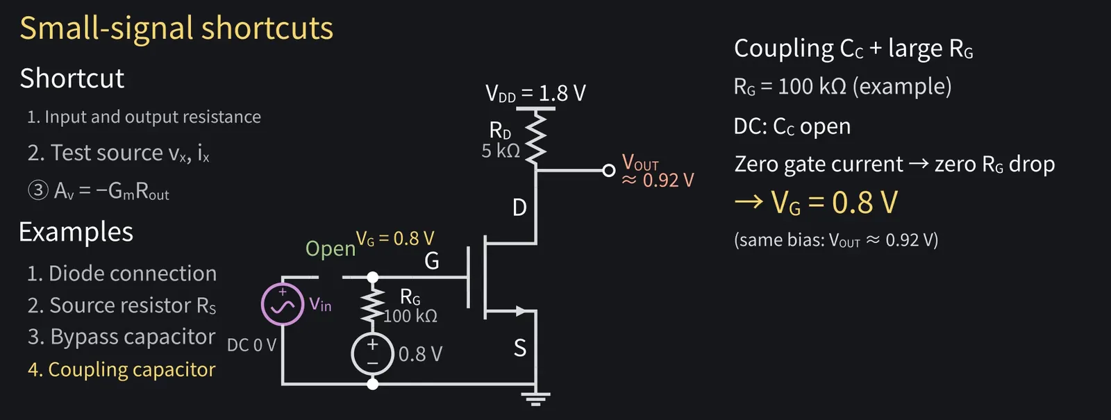
Figure 52

Shikoku Metan

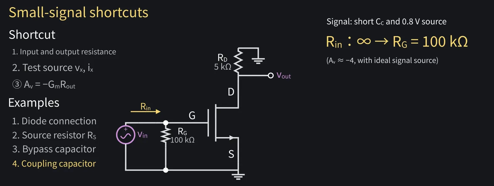
Add a coupling capacitor, and bias the gate to 0.8 V through a large resistor RG, say 100 kΩ.

Shikoku Metan: For DC, the capacitor is open. No gate current flows, so the gate stays at 0.8 V.

Illustration: For DC, the capacitor is open. No gate current flows, so the gate stays at 0.8 V.
Figure 53

Shikoku Metan

For signals, short the cap and DC source. Rin becomes RG=100 kΩ.

Illustration: For signals, short the cap and DC source. Rin becomes RG = 100 kΩ.
Figure 54

14Frequency response and SPICE AC analysis

ZundamonQuestion

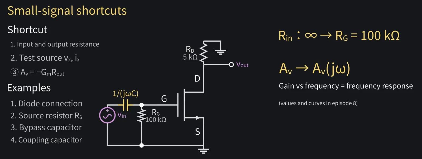
What if we keep the capacitor impedance 1/(jωC)?
Shikoku Metan

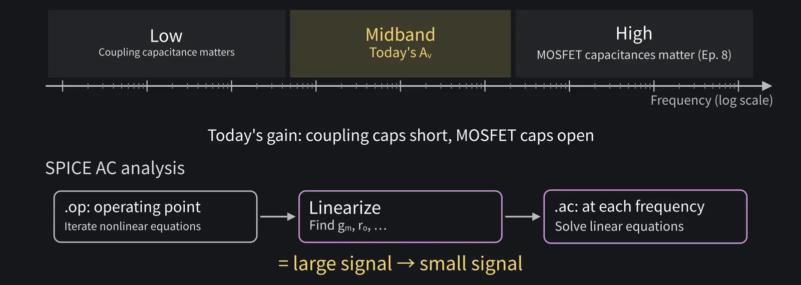
Gain varies with frequency. Plotting it gives the frequency response.

Illustration: Gain varies with frequency. Plotting it gives the frequency response.
Figure 55

Shikoku Metan

Today's gain assumes coupling caps act as shorts and MOSFET caps as opens.

Shikoku Metan: That's SPICE AC analysis: solve the linearized circuit at each frequency.

Illustration: That's SPICE AC analysis: solve the linearized circuit at each frequency.
Figure 56

ZundamonQuestion

Would a 1 V input in AC analysis distort the output?

Illustration: Would a 1 V input in AC analysis distort the output?
Figure 57

Shikoku Metan

No: it predicts an undistorted 4 V output, even though the supply is only 1.8 V. Swing and distortion need transient analysis.

Shikoku Metan: We'll cover MOSFET capacitances and frequency response in episode ten.

15Summary

Shikoku Metan

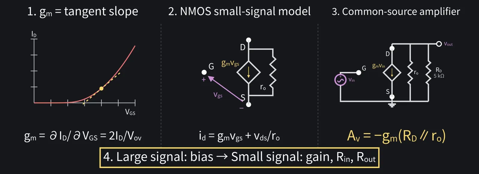
To sum up: gm is the tangent slope at the bias point.

Shikoku Metan: The NMOS model has an open gate and a gm·vgs source in parallel with ro.

Illustration: The NMOS model has an open gate and a gm·vgs source in parallel with ro.
Figure 58

Zundamon

Common-source gain is Av = −gm(RD∥ro), nanoda!
Shikoku Metan

First large signal for bias, then small signal for gain and resistances.

Illustration: First large signal for bias, then small signal for gain and resistances.
Figure 59

Zundamon

My big input violated the small-signal assumption. Now I can explain the distortion!

Shikoku Metan

Next time, let's see how to increase this gain further.

Zundamon

Thanks for reading, nanoda!